Calculate Simple Moving Average Using Google Sheets

Earlier we told you how to pull historical data in Google spreadsheet (see — HOW TO PULL HISTORICAL STOCK DATA FROM USING GOOGLE SPREADSHEET ). Once you have Historical data available in Google spreadsheet we can Calculate Simple Moving Average and values of other various technical indicators of our interest using the same.

The method given here can be used in Excel as well as Google Sheets. However we have given formulas for Google sheet. In case you wish to do same in Excel you can achieve same result by importing historical data (by Any means) and then using these formulas (some minor modification in syntax of formula may be required).

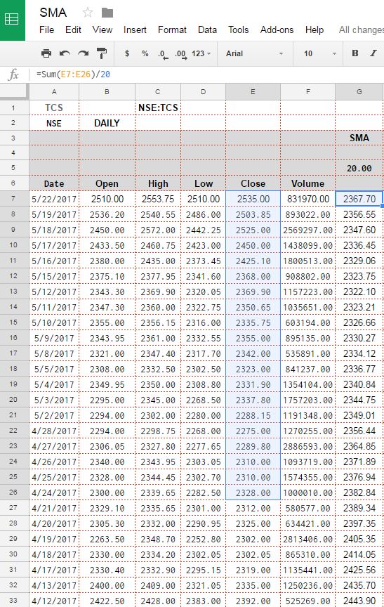
Today we are going to look how to calculate Simple Moving average or SMA for a particular period. SMA is nothing but average of last N number of Prices where N denotes the period. So if you want to calculate SMA(20,C) i.e. Simple Moving average of closing price of 20 day period. You can simply sum last 20 Close price and divide by 20, and you will get the SMA (20, C). Similarly SMA can be calculated on Open High or Low with any period, a screenshot with formula for doing so is shown below —

Problem with this method of calculation is if we need different period we will have to change the formula every time we decide to change the period. So how about a generalized formula which auto updates based on a cell where you can change the period of SMA which you want to calculate? Sound interesting?

Well this can also be done easily using OFFSET function available in both excel and Google sheet. Before we explain the function and method let’s have a look at function and values we placed for this in below screenshot.

OFFSET Function return a range of values shifted from specified position and by specified number of rows and number of columns. It can be used to return a single value or range of values. syntax of OFFSET Function is —

OFFSET(cell_reference, offset_rows, offset_columns, [height], [width])

First argument in this cell is reference from where we need to start shifting to look for target value. Second and third arguments are rows and columns that need to be shifted. It can be negative as well. Fourth and Fifth column is Height and width of range to be returned.

In our excel Fifth row mentions the period of SMA we wish to calculate. Thus using OFFSET() function and period mention in fifth row we can dynamically calculate the SMA for any period given using formula ==SUM(OFFSET(E7,0,0,$H$5,1))/$H$5.

Column E contains Closing price of share you can change it as per your excel data. Height of data is taken same as period for which SMA need to be calculated width is taken as 1 as we only need SMA of Closing price. Before doing calculation of SMA please note that if you calculating 50 day SMA you must have at least 50 Data points in historical data before the day for which you calculating SMA(50). Otherwise calculated value will be not correct.

I hope this tutorial was helpful for you all, in case of any feedback or question related to this calculation please do write in comments section and we will revert as soon as possible. In this series next we will be presenting How To calculate EMA i.e. Exponential Moving Average based on Historical data.

Link to Google sheet used in this example is — SMA Calculation sheet.